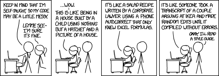
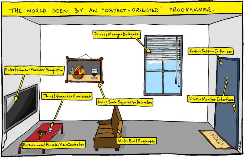
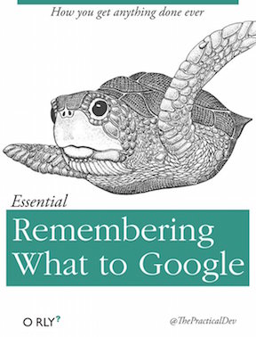
class: center, middle, inverse, title-slide # Tidy data & readable code ### Devin Judge-Lord ---  --- # R Data frames are *objects*  --- # R Resources - [Cheatsheets](https://www.rstudio.com/resources/cheatsheets/)! - Hadley Wickham on [R for Data Science](https://r4ds.had.co.nz/) - Garrett Grolemund on [R for Data Science](http://garrettgman.github.io/tidying/) - Michael DeCrescenzo on [getting started with R](https://mikedecr.github.io/811/811-basics/) - Sarah Bouchat on [getting started with R](https://bouchat.github.io/IntroDataMgmt20Jan.html) and [tidyverse and more](https://bouchat.github.io/Advanced3Feb.html) --- ## "Environment" = your current objects (data, functions, etc.) Do not "attach" data! -- ## [Read in data](https://github.com/rstudio/cheatsheets/blob/master/data-import.pdf) #### Loading saved R objects `load()` works for objects saved as .Rdata from a local file or the web #### New R objects with `readr` `d <- read_csv()` loads comma seperated values (a plain text spreadsheet) `d <- read_dta()` loads STATA data files into R (see [`haven`](https://cran.r-project.org/web/packages/haven/haven.pdf)) See this [cheatsheet](https://github.com/rstudio/cheatsheets/blob/master/data-import.pdf) for more data types and options. --- # Naming things! ## Data objects `d` for data with which you are working A more descriptive name for the original object. For example: ```{} ## Save a new object with a discriptive name regulations <- d save(regulations, file = "data/regulations.Rdata") ## Load this object as the original while we mess with "d" again load("regulations.Rdata") d <- regulations ``` `m1` or `model.1` for model output, corresponding to how you discuss them the text: "The p-value for coefficient 2 is \` r m1$p.value[2]\`." (for tidy model output) --- ## Variables **Never** use variables x1, x2 or variable1, varible2, for real data! Good names make things easy to find, recall, guess, saving you time and headaches. For Example: -- `varying` vs. `FIXED` values - A common convention, aligned with math notation Source - `values_from_dataset1` vs. `VALUES_FROM_DATASET2` - If the source is key (e.g. when joining two similar datasets) Transformations - `modified_text` vs. `Original_Text` - `modified_text <- tolower(Original_Text)` --- ### Whatever you do, use common formats **Files** (budgetEPA2016.pdf, budgetEPA2017.pdf, budgetEPA2018.pdf) **Figures** (commentsPerYear.png, commentsPerAgency.png, commentsPerAgencyPerYear.png) **Variables** (`d$commentId`, `d$commentText`, `d$commentTotal`, `d$commentUniqueTotal`) ```r starwars %>% select(name, ends_with("color")) ``` ``` ## # A tibble: 87 x 4 ## name hair_color skin_color eye_color ## <chr> <chr> <chr> <chr> ## 1 Luke Skywalker blond fair blue ## 2 C-3PO <NA> gold yellow ## 3 R2-D2 <NA> white, blue red ## 4 Darth Vader none white yellow ## 5 Leia Organa brown light brown ## 6 Owen Lars brown, grey light blue ## 7 Beru Whitesun lars brown light blue ## 8 R5-D4 <NA> white, red red ## 9 Biggs Darklighter black light brown ## 10 Obi-Wan Kenobi auburn, white fair blue-gray ## # … with 77 more rows ``` --- #[Tidyverse](https://www.tidyverse.org/learn/) ## Data manipulation with [dplyr](https://dplyr.tidyverse.org/) ### `filter` data by logical conditions ```r filter(starwars, species == "Droid") ``` ``` ## # A tibble: 5 x 13 ## name height mass hair_color skin_color eye_color birth_year gender ## <chr> <int> <dbl> <chr> <chr> <chr> <dbl> <chr> ## 1 C-3PO 167 75 <NA> gold yellow 112 <NA> ## 2 R2-D2 96 32 <NA> white, bl… red 33 <NA> ## 3 R5-D4 97 32 <NA> white, red red NA <NA> ## 4 IG-88 200 140 none metal red 15 none ## 5 BB8 NA NA none none black NA none ## # … with 5 more variables: homeworld <chr>, species <chr>, films <list>, ## # vehicles <list>, starships <list> ``` --- ### `summarize()` by group (`n()`, `mean()`, `max()`, etc.) ```r starwars %>% group_by(species) %>% summarize(species_N = n()) %>% arrange(-species_N) ``` ``` ## # A tibble: 38 x 2 ## species species_N ## <chr> <int> ## 1 Human 35 ## 2 <NA> 5 ## 3 Droid 5 ## 4 Gungan 3 ## 5 Kaminoan 2 ## 6 Mirialan 2 ## 7 Twi'lek 2 ## 8 Wookiee 2 ## 9 Zabrak 2 ## 10 Aleena 1 ## # … with 28 more rows ``` --- ### New variables with `mutate()` ```r starwars %>% group_by(species) %>% mutate(species_height = mean(height, na.rm = TRUE) ) %>% mutate(species_height = round(species_height, 1) ) %>% mutate(eye_colors = paste(unique(eye_color), collapse = ";")) %>% select(species, species_height, eye_colors) %>% distinct() ``` ``` ## # A tibble: 38 x 3 ## # Groups: species [38] ## species species_height eye_colors ## <chr> <dbl> <chr> ## 1 Human 177. blue;yellow;brown;blue-gray;hazel;dark ## 2 Droid 140 yellow;red;black ## 3 Wookiee 231 blue ## 4 Rodian 173 black ## 5 Hutt 175 orange ## 6 Yoda's species 66 brown ## 7 Trandoshan 190 red ## 8 Mon Calamari 180 orange ## 9 Ewok 88 brown ## 10 Sullustan 160 black ## # … with 28 more rows ``` --- ## `tidy()` model output with `broom` See [these slides](https://opr.princeton.edu/workshops/Downloads/2016Jan_BroomRobinson.pdf), [this vignette](https://cran.r-project.org/web/packages/broom/vignettes/broom.html), and [this example](http://varianceexplained.org/r/broom-intro/). ```r lm(height ~ mass, data = starwars) ``` ``` ## ## Call: ## lm(formula = height ~ mass, data = starwars) ## ## Coefficients: ## (Intercept) mass ## 171.28536 0.02807 ``` ```r library(broom) tidy( lm(height ~ mass, data = starwars), conf.int = TRUE ) ``` ``` ## # A tibble: 2 x 7 ## term estimate std.error statistic p.value conf.low conf.high ## <chr> <dbl> <dbl> <dbl> <dbl> <dbl> <dbl> ## 1 (Intercept) 171. 5.34 32.1 3.73e-38 161. 182. ## 2 mass 0.0281 0.0275 1.02 3.12e- 1 -0.0270 0.0832 ``` --- # Readable code Nest vs. piecemeal vs. [pipes with `magrittr`](https://magrittr.tidyverse.org/articles/magrittr.html) ### Functions can be nested ```r select( filter( filter( filter(starwars, species == "Droid"), eye_color == "yellow"), skin_color == "gold"), name, homeworld, ends_with("color")) ``` ``` ## # A tibble: 1 x 5 ## name homeworld hair_color skin_color eye_color ## <chr> <chr> <chr> <chr> <chr> ## 1 C-3PO Tatooine <NA> gold yellow ``` ### But this can be confusing and hard to edit. --- ### Instead let's define an object and modify it. ```r d <- starwars d <- filter(d, species == "Droid") ## we can streamline by "piping" d in as the first argument with %<>% ## %<>% pipes in and back out, thus modifying d, just like above d %<>% filter(eye_color == "yellow") d %<>% filter(skin_color == "gold") select(d, name, homeworld, ends_with("color")) ``` ``` ## # A tibble: 1 x 5 ## name homeworld hair_color skin_color eye_color ## <chr> <chr> <chr> <chr> <chr> ## 1 C-3PO Tatooine <NA> gold yellow ``` ### Better, certainly easier to read and edit. --- ### Now let's just pipe the object `starwars` to a series of functions with `%>%` from the [`magrittr`](https://magrittr.tidyverse.org/articles/magrittr.html) package. ```r starwars %>% ## %>% pipes one way, allowing us to string functions together filter(species == "Droid") %>% filter(eye_color == "yellow") %>% filter(skin_color == "gold") %>% select(name, homeworld, ends_with("color")) ``` ``` ## # A tibble: 1 x 5 ## name homeworld hair_color skin_color eye_color ## <chr> <chr> <chr> <chr> <chr> ## 1 C-3PO Tatooine <NA> gold yellow ``` ## Even better! --- ### Being good at R is being good at google New tasks are never easy - Google your error - Search Stack Overflow or #rstats twitter  --- # Review: Don't: - Copy and paste numbers, table, numbers, or figures into a paper - Attach data - Use `setwd()` - Use user-specific file paths (e.g. `"C:\Users\path\that\only\I\have"`) - Name files untitled.R, ProblemSet.Rmd, Rplot.png - Name variables x1, x2 or variable1, varible2, in real data - Nest when you can pipe - Write useless commit messages - Anger your future self by failing to comment your code